/data/universe/

The Best Books I Read in 2019 (and 2018)

Previous editions: 2016, 2015, 2014, 2013, 2012, 2011.

New job, new city, new kid…  I didn’t read much for a while there.  Thankfully I found Libby!

This Blessed Earth: A Year in the Life of an American Family Farm
Ted Genoways
Follows a Nebraska family as they farm corn, beans, and cattle, fighting the constant worries of weather and markets while figuring out how to pass on the business to the next generation–even as uncertainty about the future crowds in.

Our Kids: The American Dream in Crisis
Robert Putnam
A sobering study of the ever-growing chasm between the environments of kids growing up in households with and without college-educated parents in America.

The Boys in the Boat: Nine Americans and Their Epic Quest for Gold at the 1936 Berlin Olympics
Daniel James Brown
A gripping, engrossing account of the 1936 University of Washington crew which won Olympic gold in Hitler’s Germany.  Richly renders Depression-era Seattle.

Working
Robert Caro
One of the world’s greatest historians explains his craft.

Born a Crime
Trevor Noah
The South African comedian describes a childhood growing up mixed race in (post-) apartheid South Africa with humor and perception.

Digital Minimalism
Cal Newport
Digital disconnection is a luxury–but this book still offers lots of thoughtful, actionable advice about improving the quality of your life.  This blog post only exists because I deleted a bunch of apps from my phone!

Strangers in Their Own Land: Anger and Mourning on the American Right
Arlie Russell Hochschild
A Berkeley sociologist heads to Louisiana to try to understand and empathize with Tea Party conservatives.

Barbarian Days: A Surfing Life
William Finnegan
An autobiography of a life well-surfed.

Some Luck
Jane Smiley
A fictional saga follows an Iowa farm family year by year from the 1920s to the 1950s.

A Terrible Country
Keith Gessen
An American with a Russian Literature PhD on the margins of academia confronts his ideals when he moves to Moscow to care for his aging grandmother.

The Undoing Project
Michael Lewis
An intellectual biography of Amos Tversky and Daniel Kanehman, the partners who developed the broad field of heuristics and biases.

The Best Books I Read in 2016

Previous editions: 2015, 2014, 2013, 2012, 2011.

Fewer books read this year–toddlers take attention!

Twilight of the Elites: America After Meritocracy
Christoper Hayes
Perceptively anticipating current events, this book argues that America’s ostensibly meritocratic elite has become self-dealing and detached from the concerns of the larger population, undermining governance and stability.

Skyfaring: A Journey with a Pilot
Mark Vanhoenacker
A beautiful, elegiac mediation by a professional airline pilot on the human experience of air travel.

Lactivism
Courtney Jung
Examines the history, science, and sociology behind today’s widespread consensus that “breast is best.”

Water to the Angels: William Mulholland, His Monumental Aqueduct, and the Rise of Los Angeles
Les Standiford
A forgiving biography tracing the life and achievements of one of America’s great executors of public works.

Easy to Love, Difficult to Discipline
Becky Bailey
It’s challenging to read and harder to implement, but this book presents a powerful philosophy of parental discipline as teaching.

The Best Books I Read in 2015

Previous editions: 2014, 2013, 2012, 2011.

Being Mortal: Medicine and What Matters in the End
Atul Gawande
The author, a surgeon, explores how end-of-life care in the U.S. developed and why its outcomes are so often poor, as his own father nears death. He suggests that thoughtful treatment choices be guided by the patient’s reflection on a series of questions.

The Nurture Assumption: Why Children Turn Out the Way They Do
Judith Rich Harris
Research suggests that about half of our traits are inherited–children are shaped 50% by nature, 50% by nurture.  It is widely assumed that nurture means “parenting.”  In this compelling book, Harris argues that long-term parental influence (beyond genetics) is negligible.  Instead, the child’s peer group dominates.

All Joy and No Fun: The Paradox of Modern Parenthood
Jennifer Senior
Empathetic and keenly observed vignettes of parenthood in America today.

Giant Telescopes: Astronomical Ambition and the Promise of Technology
Patrick McCray
Briefly, a history of the Gemini telecopes, but really a much broader story of the evolution of optical astronomy in the U.S.  Shows how institutional tensions and Congressional fiat gave the U.S. a minority share in two telescopes rather than a true national facility.

Thank You for Your Service
David Finkel
A harrowing but important book following a group of Iraq veterans as they reenter their lives back home.

Us Conductors
Sean Michaels
Beautiful, achingly sad historical fiction about the life of the Russian Lev Sergeyevich Termin—inventor, lover, spy, and political prisoner.

Death & Co
David Kaplan, Nick Fauchald, and Alex Day
Innovative cocktail recipes and techniques from the cutting-edge New York bar.

The Old-Fashioned: The Story of the World’s First Classic Cocktail, with Recipes and Lore
Robert Simonson
A detailed history of the Old Fashioned cocktail—sugar, bitters, spirit, twist.

The Best Books I Read in 2014

Previous editions: 2013, 2012, 2011.

The Unwinding: An Inner History of the New America
George Packer
A perceptive and moving account of the recent history of the United States, told through the experiences of Americans both famous and ordinary.

Collision Low Crossers: A Year Inside the Turbulent World of NFL Football
Nicholas Dawidoff
A closely observed, richly human story that happens to be about football.  The author spent the 2011 season embedded with the New York Jets, and he draws perceptive and compelling portraits of the coaches and players as they struggle with forces outside and inside themselves, on the field and off of it.

Dad Is Fat
Jim Gaffigan
Only a professional comedian could find amusement in trying to raise five young children in a two-bedroom walk-up apartment in Manhattan.

Want Not
Jonathan Miles
Several intertwined narratives follow characters in modern New Jersey as they attempt to manage the detritus—physical, emotional, moral—filling their lives in a time of cheap abundance.

All the Devils Are Here: The Hidden History of the Financial Crisis
Bethany McLean and Joe Nocera
An exhaustive and evenhanded history of the many intertwined causes of the financial crisis.

The Two-Income Trap: Why Middle-Class Parents are Going Broke
Elizabeth Warren and Amelia Warren Tyagi
Surveys the unintended consequences of dual incomes on families with children—particularly increased bankruptcies as families overextend themselves bidding up homes in good school districts and cannot recover from unexpected events.

NurtureShock: New Thinking About Children
Po Bronson and Ashley Merryman
Summarizes unheralded but compelling recent research related to children: why some kinds of praise can backfire, the problems with giftedness tests for kindergarteners, the roots of lying and bullying, why teenagers arguing is a good thing, and more.

In a Sunburned Country
Bill Bryson
A hilarious travelogue through Australia, rendering clearly the beauty and uniqueness of the country.

Safe Baby Handling Tips
David and Kelly Sopp
Sometimes what new parents need most is a laugh.

Updated PyRAF DBSP Pipeline

When I started doing optical observing in my postdoc, I was unpleasantly surprised at how difficult it was to learn to reduce the data.  Most optical astronomers use a venerable package called IRAF, which may charitably be called “user antagonistic.”  There is a Python wrapper, PyRAF, which mutes some of the annoyances but is no easier to use if you’re not already an IRAF expert.

Using a PyRAF script originally by Branimir Sesar, I extended, generalized, and documented a pipeline (available here) for reducing long-slit spectra from the Double-Beam Spectrograph (DBSP) of the Palomar 200-inch.  It abstracts away many of the IRAF details to enable smooth reduction.  It’s useful both for quick-look classification spectra as well as moderate-precision (few km/s) radial velocity work.  Because it relies heavily on the filename and header conventions of DBSP, it would require extensive revision to use with another instrument.  However, I am advertising it in hope it will be of use to others.

The version (0.2.0) I released today overcomes several annoyances.  It automatically sets the dispersion parameters needed by autoidentify for arbitrary gratings and angles.  I’ve added a modified version of doslit to minimize repetitive prompting of the user (see here for details).  I added quicklook and batch processing scripts for fast, minimally-interactive reductions.  And I expanded the documentation, although it’s probably still not complete enough to help a true novice.

How is the US astronomy career pipeline changing?

Recently, the American Astronomical Society’s Committee on the Status of Women in Astronomy (CSWA) released a report on the demographics of US astronomers throughout the academic career cycle: graduate students, postdocs, and the various ranks of professors.  The major goal of the report (written by my friend, Prof. Meredith Hughes) was to assess the progress of women through the “pipeline” as a function of time: are women moving into the professor level in proportion to their increasing representation at the graduate student and postdoc levels, or are they “leaking out” of the pipeline?  The full report, summarized in this blog post, addresses this important question.

I was interested in a more basic question: how has the size of the pipeline itself changed over time?  That is, how many more (or fewer) grad students and postdocs are working in US astronomy compared to the number of professors over time?  The report provides proportions of the total number of men and women at each career stage by year (in 1992, 1999, 2003, and 2013), but I was curious about the totals.  Since the survey only covers a limited sample of institutions, it doesn’t represent the totality of the US astronomy job market, but it should provide a useful look.

In [10]:
%matplotlib inline
import pandas
import matplotlib.pyplot as plt
import matplotlib.pylab as pylab

pylab.rcParams['figure.figsize'] = (8, 6)

Below is the data from Figures 2 and 3 of the CWSA report. Because the 2013 report adds 8 universities and 3 research institutes to the 32 institutions surveyed in previous years, I scale the 2013 values down by that fraction. Without the raw data, it’s hard to know whether adding the additional institutions (such as Goddard) bias the career stage proportion relative to previous years. The direct scaling below should provide at least a basic level of year-to-year consistency.

In [7]:
scale_2013 = 32./(32+8+3)
df_women = pandas.DataFrame.from_dict({"year":[1992,1999,2003,2013],"grad":[176,217,269,325],
                                       "postdoc":[63,90,137,145],"assistant":[29,45,34,34],
                                       "associate":[18,37,40,44],"full":[23,37,60,71]})
df_men = pandas.DataFrame.from_dict({"year":[1992,1999,2003,2013],"grad":[602,616,549,625],
                                       "postdoc":[301,359,473,377],"assistant":[140,212,182,96],
                                       "associate":[162,220,157,187],"full":[421,511,544,426]})
df = df_men + df_women
df.index = df['year']/2
del(df['year'])
df.ix[df.index==2013] *= scale_2013
df
Out[7]:
assistant associate full grad postdoc
year
1992 169.000000 180.000000 444.000000 778.000000 364.000000
1999 257.000000 257.000000 548.000000 833.000000 449.000000
2003 216.000000 197.000000 604.000000 818.000000 610.000000
2013 96.744186 171.906977 369.860465 706.976744 388.465116

4 rows × 5 columns

In [8]:
def outside_legend():
    # Shink current axis by 20%
    ax=plt.gca()
    box = ax.get_position()
    ax.set_position([box.x0, box.y0, box.width * 0.8, box.height])

    # Put a legend to the right of the current axis
    ax.legend(loc='center left', bbox_to_anchor=(1, 0.5))

First, I plot total numbers of astronomers (men + women) in each career stage by survey year. I’ve lumped the “associate” and “full” professor categories together as “post-tenure,” although this may not be appropriate at all institutions. Note also that for research institutions, “professor” may indicate a staff position.

In [13]:
plt.plot(df.index,df["grad"],"+-",label="Grads")
plt.plot(df.index,df["postdoc"],"+-",label="Postdocs")
plt.plot(df.index,df["assistant"],"+-",label="Pre-Tenure Profs")
plt.plot(df.index,(df["associate"]+df["full"]),"+-",label="Post-Tenure Profs")
plt.ylim(0,1100)
plt.xlabel("Year")
plt.ylabel("Number in survey year")
outside_legend()

To my surprise, the number of astronomers of all career stages appears to have declined relative to a peak in the early 2000s, presumably reflecting flat funding profiles in the US and the lingering effects of the financial crisis.

Comparing raw numbers is somewhat misleading, however, as professors remain in that career stage far longer than postdocs and grad students. We can get a sense of the size of a “cohort” by dividing by a rough average number of years that astronomers remain in a career stage before moving on (or out of the academic pipeline). I have used 6 years for grad students, 3 for postdocs (although taking a second postdoc has become increasingly common in the last two decades), 7 for pre-tenure professors, and 28 for tenured professors.  Dividing by these values gives the rough number of individuals entering (and leaving, in steady state) a given career stage each year.

In [14]:
plt.plot(df.index,df["grad"]/6.,"+-",label="Grads")
plt.plot(df.index,df["postdoc"]/3.,"+-",label="Postdocs")
plt.plot(df.index,df["assistant"]/7.,"+-",label="Pre-Tenure Profs")
plt.plot(df.index,(df["associate"]+df["full"])/28.,"+-",label="Post-Tenure Profs")
plt.xlabel("Year")
plt.ylabel("Individuals per cohort")
outside_legend()

This plot highlights a large excess of postdocs in the early 2000s, presumably due to the influx of funds from to NASA’s Great Observatories (Chandra launched in 1999 and Spitzer in 2003).

Finally, we come to the sticky question: is the pipeline to professorship wider or narrower than it used to be?

Ideally, one would track a defined group through time–surveying the career outcomes of an unbiased sample of PhDs every five years, for example. The CSWA report performs survival analysis using the 1992/2003 and 2003/2013 survey pairs, but the format of the survey can’t ensure that those counted as grads or postdocs at one of the survey periods are among those being counted in the next. (A precocious senior grad student in 2003 could well be tenured by 2013, but would not be counted as “surviving” into the assistant professor stage.)

A more direct means of assessing the width of the pipeline is to compare the relative proportions of grads, postdocs, and assistant professors at each survey interval and assume a steady state. That is, if we keep graduating PhDs, hiring postdocs, and hiring assistant professors/research staff at the rate we are today, what is the oversupply ratio? This is the value most of interest to students already in the pipeline, as it indicates the amount of competition for permanent jobs. (This implicitly assumes the net flux of international astronomers into the US is zero over all career stages.)

In [15]:
plt.plot(df.index,(df["grad"]/df["assistant"]),"+-",label="Grads per new prof")
plt.plot(df.index,(df["postdoc"]/df["assistant"]),"+-",label="Postdocs per new prof")
plt.xlabel("Years")
plt.ylabel("Steady-state oversupply ratio")
outside_legend()

If we take these numbers at face value, they suggest that current postdocs face a one in four chance of getting a permanent position in astronomy, while there are more than seven current grad students for every new professor. That’s somewhat worse than implied by older data gleaned from the AAS job register (which has its own biases, particularly in undercounting postdocs). Whether this trend is real, a sampling issue, or a lingering artifact of the financial crisis is not clear.

Current and prospective students must be aware of these numbers and trends in order to be able to make well-informed career choices.   We should also improve graduate training to prepare students for a wide variety of careers, since the majority of astronomy PhDs won’t get permanent jobs in the field.  I’ll outline some possibilities in a future post.
The Best Books I Read in 2013

Following the 2011 and 2012 editions, here are the most interesting books I read this year:

When God Talks Back: Understanding the American Evangelical Relationship with God
T. M. Luhrmann
How do evangelical Christians in modern America come to believe that God speaks to them directly, as individuals? A tour de force of scholarship, synthesizing history, anthropology, and psychology, with much to offer skeptic and believer alike.

A Grand and Bold Thing
Ann Finkbeiner
A perceptive history of the Sloan Digital Sky Survey, perhaps the most successful astronomical project of all time.  Finkbeiner’s unsentimental rendering of its difficult birth is a clear reminder that science is above all a human endeavor.

The Signal and the Noise: Why So Many Predictions Fail–but Some Don’t
Nate Silver
Why are forecasts better in some fields than in others?  Silver draws examples from a wide range of fields to highlight the importance of rich data, regular feedback, and underlying causal mechanisms and the dangers of out-of-sample predictions and overfitting.

Homeward Bound: Why Women Are Embracing the New Domesticity
Emily Matchar
A balanced examination of why affluent, well-educated young women today are dropping out of the workforce and canning, growing chickens, making meals from scratch, and parenting intensively.  Aptly captures the appeal of the back-to-basics lifestyle (and the role of the Internet in promoting it) as well as potential risks for individual women and communities.

What Money Can’t Buy: The Moral Limits of Markets
Michael Sandel
Argues that the proliferation of market solutions and economic thinking is leading us astray in addressing some moral questions better determined by community deliberation.  In an age of inequality, markets do not neutrally allocate goods, and in some cases applying market logic undermines other values we would like to encourage.  Attempts to persuade gently using many real examples; some are more compelling than others.

Seven Days in the Art World
Sarah Thornton
A deftly composed series of vignettes exploring the sometimes rarefied spheres of contemporary art: auctions, art school “crits,” art fairs and biennales, studio visits, and museum prize exhibitions.  Surprisingly candid interviews with minor and very major players give perspective on the politics but also the pleasures of life in the art world.

IDL Magics for the IPython Notebook

The IPython Notebook combines code, documentation, and computational results in one package that’s easy to share.  It’s proving a great way to teach, as notebooks are easy for the instructor to write and for students to modify.  Notebooks also provide seamless integration with other programming environments through extensions providing “magic functions“: short code prefixes beginning with % or %% that call other interpreters, like R or Octave.

Since many astronomers who might want to transition to Python already know IDL, I wanted to provide an %idl magic function for IPython so they could easily call existing code.  The difficult interfacing between IDL and Python was already done by Anthony Smith‘s pIDLy package.  (As a bonus, it supports the free GDL interpreter as well.)  I adapted the Octave magic code to provide %idl magic functions with consistent syntax.  You can find the code on github as ipython-idlmagic.

The demonstration notebook below is available on github as well, or you can view it with nbviewer.

Installation

To begin, we install pIDLy:

pip install pidly

Then we install idlmagic:

In [ ]:
%install_ext https://raw.github.com/ebellm/ipython-idlmagic/master/idlmagic.py

Usage

When starting a new notebook, we load the magic:

In [1]:
%load_ext idlmagic
IDL not found, using GDL

(I am using GDL rather than IDL on this computer. idlmagic will first look for the idl interpreter on the search path and and fall back to gdl if needed.)

Line magics

The %idl magic enables one-line execution of IDL commands in the IPython interpreter or notebook:

In [2]:
%idl print, findgen(5)
      0.00000      1.00000      2.00000      3.00000      4.00000

(Note that the %idl line magic fails with TypeError: coercing to Unicode: need string or buffer, dict found in current release versions of IPython (0.13.2 and below) due to a known bug; the github development version of IPython works as expected.)

Cell magics

Multi-line input can be entered with the %%idl cell magic:

In [3]:
%%idl
x = findgen(5)
y = x^2.
; comments are supported
print, $ ; as are line continuations
mean(y)
% Compiled module: MEAN.
      6.00000

Passing variables between Python and IDL

The mechanisms for passing variables to and from IDL are based on those in the built-in %R and %octave magics.

Variables may be pushed from Python into IDL with %idl_push:

In [4]:
msg = '  padded   string   '
import numpy as np
arr = np.arange(5)
In [5]:
%idl_push msg arr
In [6]:
%%idl
print, strcompress(msg,/REMOVE_ALL)
print, reverse(arr)
paddedstring
              4                     3                     2
              1                     0

Similarly, variables can be pulled from IDL back to Python with %idl_pull:

In [7]:
%idl arr += 1
In [8]:
%idl_pull arr
In [9]:
arr
Out[9]:
array([1, 2, 3, 4, 5])

Variables can also be pushed and pulled from IDL inline using the -i (or --input) and -o (or --output) flags:

In [10]:
Z = np.array([1, 4, 5, 10])
In [11]:
%idl -i Z -o W W = sqrt(Z)
In [12]:
W
Out[12]:
array([ 1.        ,  2.        ,  2.23606801,  3.1622777 ])

Plotting

Inline plots are displayed automatically by the IPython notebook. IDL Direct graphics are used. The optional -s width,height argument (or --size; default: 600,375) specifies the size of the resulting png image.

In [13]:
%%idl -s 400,400
plot,findgen(10),xtitle='X',ytitle='Y'
% Compiled module: WRITE_PNG.

Known issues and limitations

  • The %idl line magic fails with TypeError: coercing to Unicode: need string or buffer, dict found in current release versions of IPython (0.13.2 and below) due to a known bug; the github development version of IPython works as expected.
  • Only one plot can be rendered per cell
  • Processing for possibly unused plot output slows execution
  • Scalar variables from IDL may be returned as single-element Numpy arrays

The plotting capabilities are rather kludgy due to IDL’s old-school graphics routines.  I opted to implement Direct Graphics, which are the lowest common denominator supported by IDL and GDL.  Since I have to initialize the device before the plot call and close it afterwards, the %idl magic can only produce one plot output per notebook cell.  The plotting code produces overhead on non-plotting lines as well, unfortunately; I chose syntactic simplicity over execution speed for the time being.

Stay tuned to see it in action!

Bitten by Sample Selection Bias

At this week’s meeting of the High Energy Astrophysics Division of the American Astronomical Society, I learned that one of the teams analyzing data from a NASA observatory had run into trouble with their machine learning classifier.  Their problem illustrates one of the particular challenges of machine learning in astronomy: sample selection bias.

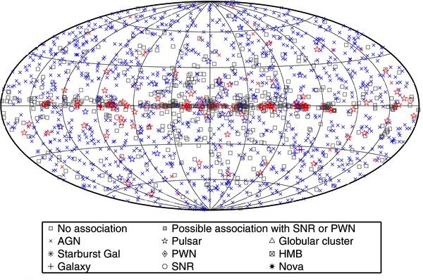
All-sky map of Fermi sources (Nolan et al. 2012).

All-sky map of Fermi sources (Nolan et al. 2012).

At first glance, it looks like a classic machine learning problem.  The Fermi Gamma-Ray Space Telescope has performed a highly sensitive all-sky survey in high-energy gamma-rays and detected nearly two thousand sources, most of which are unidentified.  It’s expected that most of these will either be pulsars–rapidly-rotating neutron stars–or active galactic nuclei (AGN), accreting supermassive black holes in distant galaxies.  Many teams (including one I work with) are interested in detecting the Fermi pulsars in radio or optical bands.  We’re interested because many of these pulsars proving to be rare “black widow” systems, where the pulsar in the process of destroying its low-mass companion and it is possible to determine the mass of the neutron star.  However, telescope time is precious, so there needed to be a way to prioritize which systems to follow up first.

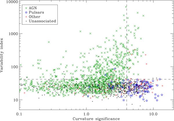
The pulsars and AGN are distinguished by their variability in the gamma-ray band and by the presence or absence of curvature in their spectra.  It seems obvious, then, to train a classifier on the data for the known systems and then use it to predict the class of the unknown systems, and several groups did just that.

Spectral curvature vs variability for Fermi sources by source class (Nolan et al 2012).

Spectral curvature vs variability for Fermi sources by source class (Nolan et al. 2012).

However, when the Pulsar Search Consortium searched the newly-prioritized list, they found fewer new pulsars, not more.  The problem turned out to be a bias in the training set: the known sources used for training are brighter than the unknown ones being predicted.  In this case, the major effect was that the fit of the spectral curvature was inconclusive for dim sources–there weren’t enough counts to tell a curved line from a straight one, so the features fed into the classifier weren’t reliable.  As usual, garbage in, garbage out.

In astronomy, this situation is quite frequent: the “labelled data” you’d like to use to train a classifier on is often systematically different from that which you’re trying to classify.  It may be brighter, nearer, or observed with a different instrument, but in any case blindly extrapolating to new regimes is unlikely to yield reliable results.  Joey Richards and his collaborators describe this problem of sample selection bias in great detail in their excellent paper, where they focus on the challenge of classifying different types of variable stars from their light curves.  They find that iterative Active Learning approaches are most effective at developing reliable classifiers when the unlabelled and labelled data may be drawn from different populations.  In Active Learning, the classifier identifies the unlabelled instances whose classification would most improve the performance of the classifier as a whole.  These targets can then be followed up in detail, classified, and the process repeated.

This approach worked well for variable star problem, where the features used in the classifier were valid for all the sources.  For the Fermi problem, the challenge is that one of the most informative parameters is unreliable for a subset of the sources.  In this case it might be more useful to develop additional features that might identify spectral characteristics even in the low-flux regime.

Making Space in LaTeX Documents

A recent major proposal deadline gave me a chance to brush up on my LaTeX skills. As a rule, it’s better to make your proposal more concise than to play formatting tricks to squeeze more text in. For this proposal, though, I needed the big guns–for some sections the instructions alone were a significant fraction of the allotted space! Below are some tested methods for cramming more material into your page limit:

  1. Choose your text size. As a first step, be sure your text is set to the minimum allowed point size.
    \documentclass[11pt]{article}
  2. Get the margins right. The geometry package provides the easiest means to specify margins.
    \usepackage[paper=letterpaper, margin=1in, 
           nohead, pdftex]{geometry}

    If there aren’t firm margin requirements, the fullpage package is an alternative:

    \usepackage[cm]{fullpage}
  3. Compress your lists. Standard LaTeX list environments leave lots of whitespace between the items. The paralist package provides compactitem and compactenum, drop-in replacements for itemize and enumerate.
    \usepackage{paralist}
    
    \begin{compactitem}
    \item Item text.
    \end{compactitem}
  4. Use runin headers. If your document is of any length, it’s helpful to organize it into parts, sections, subsections, and possibly even subsubsections. Standard LaTeX classes give each of these large headings on their own lines. The titlesec package provides an alternative: run-in headers. These appear in-line in the text, saving space. You can adjust the format and numbering with the \titleformat command. The commands below set up small-caps part headers on their own lines (“hang”), and variously sized run-in bold headings for sections.
    \usepackage[compact,medium]{titlesec}
    \titleformat{\part}[hang]
    {\Large\scshape}{}{0pt}{}
    \titleformat{\section}[runin]
    {\large\fontseries{b}\selectfont\filright}{}{0pt}{}
    \titleformat{\subsection}[runin]
    {\normalfont\fontseries{b}\selectfont\filright}{}{0pt}{}
    \titleformat{\subsubsection}[runin]
    {\fontshape{it}\selectfont\filright}{}{0pt}{}
  5. Use superscript citations. If your field allows it, no citation notation uses less space than superscripted numbers. The natbib package makes it easy.
    \usepackage[super,sort&compress]{natbib}
    \bibpunct{}{}{,}{s}{}{,}
  6. Put captions beside floats. Figures and tables can end up with unused whitespace on the sides. The excellent LaTeX Wikibook provides several suggestions, including using the wrapfig package to wrap the text or using a minipage or the sidecap package to move the caption beside the text. I have used floatrow to accomplish the same task:
    \usepackage{floatrow}
    
    \begin{figure}
    \floatbox[{\capbeside\thisfloatsetup{capbesideposition={right,center},capbesidewidth=0.46\textwidth}}]{figure}[\FBwidth]
    {\caption{
    {\small
    Caption text here.
    \label{fig:myfig}
    }}}
    {\includegraphics[width=0.52\textwidth]{myfig.pdf}}
    \end{figure}
  7. Single-space the bibliography. The code below removes the bibliography section label and single-spaces the entries: put it in the document header.
    % no title on bibliography header: this duplicates the section of
    % article.cls, removing the refname section
    \makeatletter
    \renewenvironment{thebibliography}[1]{%
    \list{\@biblabel{\@arabic\c@enumiv}}%
    {\settowidth\labelwidth{\@biblabel{#1}}%
    \leftmargin\labelwidth
    \advance\leftmargin\labelsep
    \@openbib@code
    \usecounter{enumiv}%
    \let\p@enumiv\@empty
    \renewcommand\theenumiv{\@arabic\c@enumiv}}%
    \sloppy
    \clubpenalty4000
    \@clubpenalty \clubpenalty
    \widowpenalty4000%
    \sfcode`\.\@m}
    {\def\@noitemerr
    {\@latex@warning{Empty `thebibliography' environment}}%
    \endlist}
    \makeatother
    
    % make bibliography single-spaced
    \let\oldthebibliography=\thebibliography
    \let\endoldthebibliography=\endthebibliography
    \renewenvironment{thebibliography}[1]{%
    \begin{oldthebibliography}{#1}%
    \setlength{\parskip}{0ex}%
    \setlength{\itemsep}{0ex}%
    }%
    {%
    \end{oldthebibliography}%
    }
  8. Use or make a compact bibliography style. Exclude anything you can from the reference list. I made a BibTeX style file which defaults to “et al.” anytime there is more than one author.
  9. Discourage floats from getting their own pages. LaTeX uses a number of numeric weights to calculate where to position floats. Fiddling these parameters in the document header will encourage LaTeX to place them closer to each other and the text.
    % discourage floats from getting their own page
    \renewcommand\floatpagefraction{.9}
    \renewcommand\topfraction{.9}
    \renewcommand\bottomfraction{.9}
    \renewcommand\textfraction{.1}   
    \setcounter{totalnumber}{50}
    \setcounter{topnumber}{50}
    \setcounter{bottomnumber}{50}
    
    % shrink space between/after figures:
    \setlength{\textfloatsep}{10pt plus 1.0pt minus 2.0pt}
    \setlength{\floatsep}{10pt plus 1.0pt minus 2.0pt}
    \setlength{\intextsep}{10pt plus 1.0pt minus 2.0pt}
  10. Vacuum up the extra whitespace. Several more header parameters adjust white space between document elements.
    % Reduce space between section titles
    % Arguments are space before, vertical space, and space after
    \titlespacing{\part}{0pt}{*0}{2ex}
    \titlespacing{\section}{0pt}{2pt}{1ex}
    \titlespacing{\subsection}{0pt}{2pt}{1ex}
    \titlespacing{\subsubsection}{0pt}{*0}{1ex}
    
    % suck up extra white space
    \setlength{\parskip}{0pt}
    \setlength{\parsep}{0pt}
    \setlength{\headsep}{0pt}
    \setlength{\topskip}{0pt}
    \setlength{\topmargin}{0pt}
    \setlength{\topsep}{0pt}
    \setlength{\partopsep}{0pt}
  11. Encourage paragraphs to consolidate words on their own lines.  Individual paragraphs can be tweaked with
    \looseness=-1

    or simply set

    \linepenalty=1000

    at the beginning of the document.

  12. (Adjust or remove indentation.) Changing the paragraph indentation level can recover a few characters, but it makes the text harder to scan.
    \setlength{\parindent}{0in}
  13. (Black Hat: Shrink the inter-line spacing.) While I’m not comfortable with this measure and it makes the text hard to read, it is possible to make the line spacing less than one.
    \linespread{0.8}


As usual with LaTeX, there are multiple ways to accomplish the same goals–these are methods I personally have found convenient. The savetrees package provides an all-in-one solution which may be sufficient if you don’t want to tune the document style yourself.