/data/universe/

The Data Science Core Curriculum

Jake Klamka spoke at Caltech a few months back about his Insight Data Science Fellowship–a program designed to help science PhDs transition into jobs in data science.  The program guides scientists in packaging skills they already have so that employers can easily see the relevance and value to their business.  Jake’s own initial difficulty getting a tech job inspired the program–after working as a particle physicist, he didn’t have any resources to help him determine which skills were important to learn and to help him get unstuck when he had problems.

There is no standard data science job, so there isn’t a standard set of skills for data scientists.  Still, Jake identified a common set of basic skills for scientists to build first as a foundation:

  • Python.  In many ways the lingua franca of programming today, Python is an excellent all-in-one tool for everything from scripting to web programming to statistical analysis.  R is a useful second language.
  • Databases.  SQL is a must.  The Hadoop ecosystem is important, but it’s probably more practical to learn on the job.
  • Visualization, particularly with d3.js. Scientists understand the importance of visualization in making sense of data; d3 is a modern, web-first framework for building interactive visualizations.  (Bonus: it helps you learn some JavaScript.)
  • Computer Science fundamentals–Most scientists have no formal CS training, but knowledge of basic algorithms and data structures is vital for working with large datasets.
  • Machine Learning–A high-level understanding of what’s possible will let you get started.

To these, I might add familiarity with the basic tools of software development (“software carpentry“), particularly version control and unit testing.  Scientists presumably have ample experience with statistics and quantitative methods.

Data science in practice encompasses a huge and growing range of tools and techniques, but this core curriculum provides a manageable start.  We live in a fortunate time–there are many excellent free online courses so you can learn these skills now, on your own time–and they’ll even be valuable in your current academic job!

Tracing the Changing State of the Union with Text Analysis

U.S. Presidents since George Washington have delivered State of the Union addresses each year to describe the nation’s condition and prioritize future action.  Can we glean historical patterns from the texts?  Do presidents speak similarly in times of war or depression?  Do Republicans and Democrats emphasize different words?  How does the evolution of American English affect the speeches?

To explore these questions, I performed textual analysis of all of the State of the Union Addresses given through 2012.  (For those interested, technical details are at the end of the post.)  I broke the addresses into words, removing words like “the” and “and” and weighting uncommon words more highly.  Then I measured the similarity of each pair of presidents by counting the words they used in common.

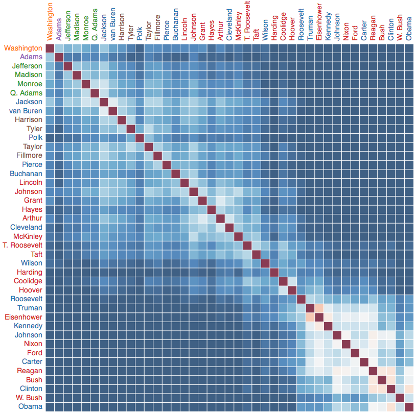
This figure shows the pairwise similarities for presidential State of the Union addresses–click for an interactive version.  Blue squares indicate that the presidents used few words in common, while white and red imply more overlap in vocabulary.  The red diagonal line is the similarity of each president to himself, which is obviously 100%.  I’ve color-coded the presidents by their political party.

Several interesting trends appear.  First, the dominant effect is that presidents nearer in time use more similar words.  Second, there seems to be a general separation before and after the early part of the 20th century (Wilson-Hoover): there is a great deal of overlap among the early presidents and among the post-WWII presidents, but less similarity between those groups.

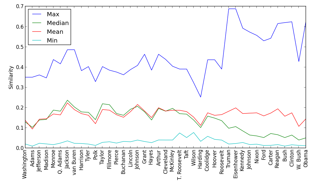
We can look for bulk similarity and difference by aggregating the similarities for each president and looking at the range of values (excluding the self-comparison):

Few presidents seem to generate unusual influence on later addresses.  However, some presidents use noticeably different language than their peers, including John Adams, James Polk, Warren Harding, and George W. Bush.

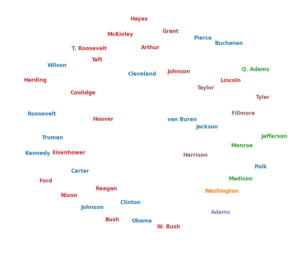
Finally, each president’s words define a direction in vocabulary space.  We can project the presidents’ addresses into two dimensions, spacing the points by their relative distances in vocabulary space:

Closer presidents in this projection are more similar, so we can easily see that temporal order rather than political party seems to be the dominant effect influencing the language that presidents use in their State of the Union addresses.

Read the rest of this entry »

Python for IDL Users I: Ecosystem

Python is often the language of choice for today’s cutting-edge astronomical software.  Scientists wishing to take advantage of this powerful and growing ecosystem face the hurdle of learning a new programming language.  Thankfully, with the rapid growth of scientific Python, a number of excellent comprehensive tutorials have been developed, many particularly for astronomers:

All of these are great resources for getting up to speed in Python.  Here, I’d like to cover similar ground (installation, packaging, language features, etc.), but focusing explicitly on how Python differs from the language most astronomers know best: IDL.  My hope is that direct comparison and contrast with a familiar language will make the learning curve easier.

Installation

The installation process for IDL is more straightforward than that of Python, and that fact likely deters busy scientists from even giving Python a try [1].  IDL programs run on  a proprietary interpreter sold by RSI ITT Exelis.  Accordingly, your system administrator has to manage software licenses, so they have likely already installed IDL on public servers and maybe even set your IDL_PATH to point to the IDL Astronomy User’s Library.  In this case, you don’t install IDL at all!  Likewise, installing IDL on your laptop generally just requires a simple point-and-click installer, configuring a license file, and setting your IDL_PATH to point to appropriate libraries, which are just directories of IDL programs.

Python, in contrast, is free software that is under active development.  Moreover, the packages useful for science are not part of the core language runtime and are developed independently.  This situation is an advantage for Python insofar as it enables a broad software ecosystem, but it makes installation more complex.  (Also, Python packages often glue in existing C, C++, and FORTRAN libraries which need to compile during installation.)

One additional complication–hopefully to resolve itself naturally soon–is the Python version split.  Python 3 introduced backwards-incompatible changes to the language.  Since most of the power of Python is in the external packages, scientific migration to Python 3 has been slow.  Accordingly, for now it’s best to continue working in Python 2.7 (the current and final pre-Python 3 release) rather than Python 3.3 (the newest version).

There are several methods of installing Python and its external packages on Mac OS X and Linux; I have ordered these roughly by popularity.  (I don’t have enough experience with Python on Windows to make recommendations.)

  • Use a package manager.  In my opinion, this is the best choice for long-term Python use.  Mac OS X programs like Macports (or familiar Linux equivalents like apt-get or yum) make it easy to keep installed packages up-to-date.  These work primarily on the command line (and install non-python software as well).  You choose which packages to install (e.g., sudo port install py27-numpy), and at later times a simple sudo port selfupdate command will bring all of your libraries up to date.  The package manager handles all the tricky details of library dependencies, compilers, and paths for you.  An excellent step-by-step guide for installing astronomical python via Macports is here.
  • Use an all-in-one installer.  Many astronomers appreciate the one-click convenience provided by the Enthought Python Distribution (EPD) [2], which bundles together many (but not all) of the major scientific python libraries.  I have personally found it convenient for getting a new version of python on shared servers where I didn’t have root access.  However, EPD costs $199 for a single-user license.  While this fee supports further Python development, it means that the EPD distribution requires license files, even for the free version offered to academics.  My experience has been that this licensing complicates upgrading packages or EPD itself and negates Python’s advantage of being free to install on all of your systems.
  • Maintain your installations manually.  It’s possible–but far more complicated–to maintain your packages manually.  Manual installation isn’t beginner-friendly, though–not all programs are packaged in the same way, and you have to manage dependencies, upgrades, and paths yourself.  If you go this route, pip is currently the installation method of choice, and virtualenv is recommended to create isolated Python environments.  See the installation section of this guide for more tips.
  • Use the built-in system Python.  Not recommended!  While both Mac OS X and Linux are likely to have system versions of Python installed, they may change in system upgrades and break your code.  Moreover, the packages you install may cause conflicts with routines your computer depends on.  However, if you just want to play with the language, though, simply typing python in a terminal will give you a way to start.

Next time: IDL and Python, head to head!

Getting a new OS X Finder window in the current Space

Mac OS X provides multiple desktops via the Spaces feature.  I use this feature all the time to keep my mental workspace uncluttered: typically I have one Space with a web browser, one or two more with terminals (iTerm2 is great), and another with documents or presentations.

In Apple’s Spaces model, if you click on the icon of an already-running program in the Dock, it takes you to the Space where that application’s windows are.  For example, if I’m in Space 3 and have iTunes open in Space 1, clicking the iTunes icon will move me to Space 1.

This automatic space-switching behavior is not what I want with Finder.  When I click on the Finder in the Dock I want a new Finder window in the current space.  What happens instead is unpredictable.  If I have no Finder windows open in any space, I get what I want:  a new Finder window where I am now.  However, if I have forgotten Finder windows in other Spaces, OS X will zip me away from what I’m doing to those old Finder windows.  That unexpected switch destroys whatever sense of flow I have as I drag back to my current Space.

Two methods for getting a new Finder window in the current space don’t work well for me personally.  The first is to right click on the Finder icon in Dock and select “New Finder Window.”   The second method is to switch to Finder (either by Cmd-Tab or by clicking on the desktop), then hitting Cmd-N.  Both methods are too cumbersome for me, though they might satisfy you.

Instead, I found an Applescript method to produce a new Finder window.  I modified the code slightly to give focus to the new window and to start in my chosen directory:

on run
tell application "Finder"
set NewWindow to make new Finder window
set target of NewWindow to "Macintosh HD:Users:username:path"
activate
end tell
end run

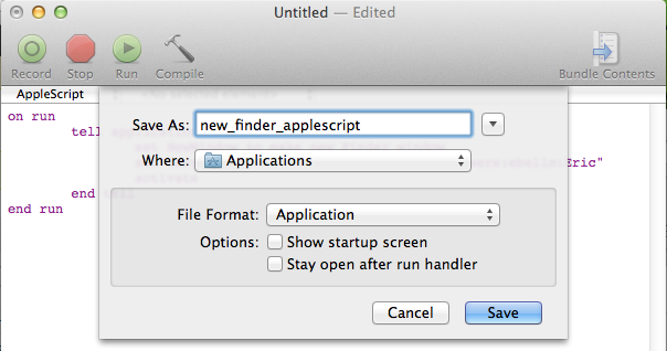
Open AppleScript Editor (via Spotlight is easist) and paste in the code.  (Replace username with your username and the path as well.)  Save the file as something like new_finder_applescript in your Applications folder.  Set the format to Application and make sure that “Stay open after run handler” is unchecked.

Next, let’s replace the default applescript icon with something better.  I like this CC-licensed Finder icon by Gordon Irving.  Download the .icns version.  Open your Applications folder and Cmd-click on new_finder_applescript and select “Get Info.”  In the top left will be the default “rolled paper” Applescript icon.  Drag and drop the new icon file onto the default icon…

and the new icon should appear.

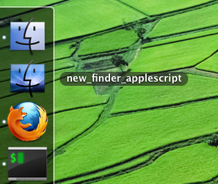
Finally, drag the new_finder_applescript icon into the Dock.  I like to place it just below the standard Finder (which can’t be removed from the Dock without terminal hacking).

Now, a quick click on your new icon will give you a Finder window in the current Space, no matter what!  It’s possible to bind your script to a hotkey with third-party programs like Quicksilver or FastScripts as well.

Four Short Links: An Appreciation

Twitter, Prismatic, Google Reader, and Hacker News keep me up to the minute on the tech news I care about.  While I tune my feeds to give me more signal and less noise, popular links frequently repeat: five people I follow on Twitter link to a story, then I find it on top of my Prismatic feed, and later it’s on the front page of Hacker News.

I therefore treasure orthogonal sources that break out of that echo chamber.  The “Four Short Links” series on the O’Reilly Radar blog is one of my favorites.  Every day Nat Torkington offers four links to under-the-radar news items joined with description and commentary of masterful brevity.  It holds pride of place among my RSS subscriptions; maybe you’ll like it, too.

Scientists: Career Change Starts Now

Jessica Kirkpatrick wrote a great post describing her move from astronomical research to a data science job at Yammer.  (We were classmates in grad school.)  She discusses the technical skills she needed to learn (IDL alone won’t get you a tech job) as well as the differences between business and academic culture.  (Peter Fiske’s book Put Your Science to Work can help guide scientists through that cultural translation.)

In the comments, a finance recruiter added a key point:

The only thing I would add is come prepared to explain your motivations for wanting to move to industry. It’s important you can convince your future employer that you are moving for the right reasons.

I’ve heard that refrain a lot lately:  from panelists discussing aerospace careers for astronomers at the AAS meeting, from Jake Klamka of the Insight Data Science Fellowship, from professors describing jobs at teaching-focused colleges.  Apparently it’s surprisingly common for scientists to come into interviews with an attitude of “My research funding ran out, but I’m super smart and ready to make some real money.  What do you do here again?”

Obviously that approach insults your potential coworkers.  It’s far more productive to demonstrate your enthusiasm for the job and the goals of the company.  The more your background differs from the job you’re applying for, the more effort you need to make to show those hiring that you can do the job and that you’ll fit in the company culture [1].

One of the staples of interview advice is to substantiate your claims with stories.  Accordingly, the best way to show your interest in your new industry is to point to previous work you’ve done in the field!  That could be an internship or volunteer work, a side project you did on your own time, a subject-focused blog you maintain, or attendance at a conference or meetup group.  (These explorations will also help you confirm your interest in the industry.)  Thus, smooth career changes out of academia begin with groundwork laid well before you actually change fields.

For data science, it’s particularly easy: as Hilary Mason points out, you can start doing data science right now!  There are many publicly-available datasets and apis, and many of the standard tools are open-source.  Brush up on your machine learning and join a Kaggle competition, or try making an engaging visualization.  Creative projects are fun, teach you new skills, and make you an easier hire all at once!

Ideas for Improving Your Scientific Visualizations

Scientific graphics are one of the most important means we have of communicating complicated quantitative information.  Here are a few ideas for improving the effectiveness of your figures:

  • Learn a new feature of your graphics package.  Most of us only use a fraction of the capabilities of our graphics programs.  There’s much to be gained from digging around in the documentation.  Users of python’s matplotlib might want to play around with the AxesGrid toolkit, learn about animation or widget capabilities, or look through these recipes.  IDL users could define more sensible plotting defaults.
  • Read a book.  Edward Tufte’s Visual Display of Quantitative Information is rightly a classic.  Its principles for evaluating the information density of figures will change how you think about graphical communication.  Nathan Yau‘s Visualize This (and his website, FlowingData) provide a look at today’s cutting edge of information graphics.
  • Learn about color perception.  Scientists love rainbow colormaps.  However, rainbow colormaps create perceptual artifacts that obscure the very trends you’re trying to display.  Perceptual colormaps are a better alternative.  The ColorBrewer colormaps are the most well-known.  Python’s matplotlib has them built-in (try help(plt.colormaps)), and versions are available for IDL as well.
  • Use alpha transparency.  Most modern graphics packages support semi-transparent elements via an alpha keyword, typically specified between 0.0 (completely transparent) and 1.0 (completely opaque).  Making lines or scatterplot points semi-transparent can improve the clarity of the plot if there is overlap or variation in point density.
  • Learn about web visualization.  Static figures aren’t going anywhere–they’re easy to print, share, and display on slides.  However, both the true day-to-day practice of science and the needs of large datasets require an exploratory approach to visualization.  Interactive analysis needs sophisticated software, however.  The most nearly universal means to share interactive visualizations is via the browser, with its widely available JavaScript runtime.
    Today, the d3.js library is the most popular JavaScript visualization library.  It is hugely capable, though with its power comes complexity.  Check out an online tutorial or a book to get started.

When Facebook was Fun

It’s hard to remember, now, but there was a time when Facebook was the most exciting thing on the Internet.

I was a junior at Harvard when thefacebook.com [1] started in February 2004, but I didn’t sign up when I first heard about it.  Since I had the relatively uncommon habit of reading The Crimson over breakfast, I knew about the
trouble Mark had gotten into for Facemash, the “Hot or Not” site he’d built by scraping student id photos from the websites of the undergraduate Houses.  When I heard he had opened a Friendster-like site for Harvard students, I decided to wait and see.

Others were more adventurous.  One of my physics classmates was sitting at his email (Pine, of course) when Mark sent the announcement to the list for AEPi, the Jewish fraternity [2].  He signed up, earning himself a user id number under 10.  I held out for three or four days until my coolest friend sent me an  invitation to join [3].  By that point already more than 1100 people had joined.  By the end of February, essentially everyone at Harvard was on.

Once signed in, it was easy to see what the excitement was about.  While the site was very simple, there was an immediate rush to see what your friends were writing and to show off your most interesting self.  Which books should I list to show off my literary sensibilities?  Which forgotten philosopher should I quote?  Should I include obscure bands, or embarrassing pop, or both?  [4]

In the beginning there was only a static profile page with your picture and a number of text fields for your House, hometown, interests, favorite books and music, etc.  No photo albums, no News Feed, no status updates; I don’t even remember if there was private messaging right away.  There was a Wall, but it was a simple text field that your friends could edit.  Only the last person to make a change was noted underneath.  And there was Poking–a vaguely naughty digital ping whose yet-undetermined social norms made it all the more interesting.
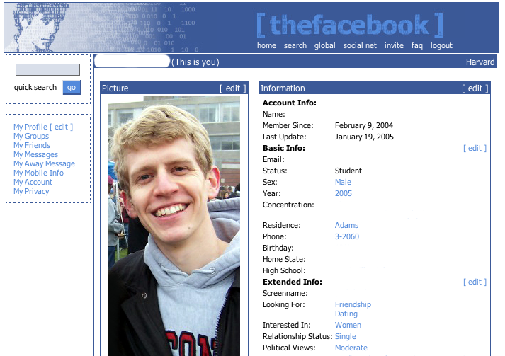
Facebook Profile, early 2005

My Facebook profile, early in 2005. Click to see the rest of my carefully curated interests.

You could browse the list of your friends’ friends, and every profile listed the number of friends you had.  That quantification was a source of some angst in the early going, when it really was connected to the size of your social circle on that ambitious campus.

From today’s perspective, thefacebook was surprisingly private.  You could only see someone’s profile if you were friends, and you could only get an account if you had a harvard.edu email address.  That restriction was a big part of Facebook’s initial success–people were willing to create profiles because only their peers would see them, in contrast to Friendster or Myspace.  And Harvard students love to be told they’re special and to be given exclusive access.

In those early days, you added new friends as more people joined, obsessively monitored your friends’ profiles for changes [5], and continually tweaked your profile.  There was a page that showed which of your friends had recently updated their profile, but you still had to figure out what was different [6].  There was an arms race be the most clever within the constraints of the medium.

About the time we started getting the hang of thefacebook, Mark begin expanding to other colleges–first Yale, then Stanford, and so on down the line of the U.S. News and World Report rankings.  At first you couldn’t even friend people in other college networks, but that soon changed [7].  Still, for all intents the networks were separate.

Groups were imagined as ways for athletic teams and clubs to connect, but they quickly became another way to display your creativity and personality by showing solidarity with an idea.  One of the most popular early groups at Harvard was “I Went to a Public School… Bitch”, signaling to all those elite toffs that you were from the mean streets of Naperville [8].

As more schools were added, there was a fertile cross-pollination of the new digital culture across campuses.  Student newspapers across the country grappled with the meaning of the poke.  Chapters of popular Groups sprouted up in each campus, and jokes and references proliferated in patterns of viral remixing which now seem commonplace [9].

That summer, Mark went off to California.  He never came back, except to recruit.  Facebook was never really ours again.

Perhaps surprisingly, very few of my classmates went to work for Facebook.  In those days investment banking was viewed as the sure path to riches.

I’ve been calling him Mark here, quite familiarly, but I never knew Mark personally.  I did take a gut (an easy course) with the brothers Winklevoss.  I knew back then about the founding drama and ConnectU from the Crimson, and I’m certain that the brothers couldn’t have made Facebook Facebook.  Part of Facebook’s appeal in those first days was that it was clean, protected space very different from the all-too-public hurly-burly of MySpace [10]. Mark’s technical instincts were vital to Facebook’s early success [11].

The rest of the story you know.  Facebook continued to grow, bringing in first high-schoolers, then companies, then everyone.  The boundaries between networks slowly dissolved, and the default sharing settings slowly widened.  The introduction of Photos and friend-tagging provided some reinforcement for offline interactions, but the general trend was toward more generic, global sharing.  People began to worry about their privacy settings as their words and actions became exposed to outside eyes: family members, old acquaintances, employers.

And we grew older.  The guy who was your buddy in class or in the dorms moved to a different city, and you lost touch with him, except in the weird limbo of Facebook, where you remain capital-F Friends and your seven-year-old inside jokes remain preserved in digital amber.  You don’t notice it, as the News Feed pushes your recent history out of sight, but who you were trying to be back then can still be found in your Timeline.  What was once a means of creative expression and a connection to a living community has ossified: a hidden record of who you aspired to be, as you became who you are now instead.
The Best Books I Read in 2012

Following the 2011 version, here are the best books I read this year.

Moonwalking with Einstein
Joshua Foer
Can a normal person become a memory champion?  Joshua Foer covers a lot of ground in this well-written book, including extensive historical background as well as considerations of neuroscience, deliberate practice and expertise, savantism, and immersive journalism.

How I Killed Pluto and Why It Had It Coming
Mike Brown
A funny and very humanizing picture of a scientist at work: A great account of the quest to discover planets beyond Pluto, and of the upheaval that followed.

The Perfect Machine
Ronald Florence
The epic story of the building of the 200-inch Palomar telescope, for nearly half a century the largest in the world. It was made into a PBS special which is available online.

Steal Like an Artist: 10 Things Nobody Told You About Being Creative
Austin Kleon
Previously recommended: A pithy but rich collection of tips for nurturing creative projects.

The Management Myth
Matthew Stewart
A critical history of management theory and education from Taylor to present MBAs, with humorous stories from the author’s consulting career interspersed.  Stewart’s main contention is that there is no “science” of management, and attempts to create one are actively harmful.

Lightning Rods
Helen DeWitt
The plot synopsis for this novel is so ribald that it’s risky (and risqué) to recommend, but the careful reader will find here a subtle but oh-so-sharp satire of business self-help and evolutionary essentialism. Funny, too.

The Sense of an Ending
Julian Barnes
This novella, winner of the 2011 Man Booker Prize, is an extended meditation on memory and responsibility.  Its hidden depths had me repeatedly rereading key passages looking for clues.

The Cult of Personality Testing
Annie Murphy Paul
Describes the origins, motivations, and limitations of widely-used personality tests, pointing out that the popular attempts to label people into “types” or discern features of their personality are generally unscientific and overapplied.  The Rorshach, Myers-Briggs, MMPI, TAT, and others have colorful histories, but their accuracy and utility are far less than assumed.

Outside Lies Magic: Regaining History and Awareness in Everyday Places
John Stilgoe
Stilgoe, a Harvard professor of Landscape History, shows the pleasures and insights gained by exploring seemingly ordinary places (residential subdivisions, small-town Main Streets, highway interchanges) on foot or bicycle with an eye for detail.  He unearths historical clues and patterns from eras past in the built environment: why Main Street has a unified architectural style of brick, why hobby shops and antique stores flourish on in old downtowns, how rail right of ways determined the layout of towns and cities.

Minimal Mercurial

As a scientist, most of my work consists of text files: source code, data, and papers. Keeping track of changes to these files with version control helps me avoid losing work, track down bugs, reuse code, and keep records of my research. Rather than renaming files code.py.oldversion, code.py.aug01, code.py.brokendontuse, version control gives me a single, current source file as well as a database of changes that I can use to restore any previous version at will.

Older version control programs (e.g., CVS, SVN) were designed for large teams collaborating on a single code base, so they store changes in a single, centralized repository. For the solitary scientist, newer “decentralized” version control systems like Git and Mercurial work better: they are lightweight and easy to set up, and since the entire change history is carried with the code, it’s easy to keep your work synced across multiple computers.

Among software engineers, Git is far more popular than Mercurial, thanks largely to the online repository github [1]. Git is unnecessarily complicated for most of the work I do, though, so I prefer Mercurial for day-to-day use.  With either system, though, a single scientist only really needs a few simple commands to get most of the benefits of version control.  The Win-Vector blog published a guide for git; here is mine for Mercurial.

After installing Mercurial [2], typing hg at the command prompt should print a list of basic commands [3].  Of these, three are the most used:

hg init
hg add <filename or pattern>
hg commit

hg init creates a new respository in the current directory.  You only need to run it once, when you first start tracking files for a project.  It creates a hidden directory .hg in the current directory to store changes in.

hg add <filename or pattern> tells Mercurial to track changes for the specified files.  Again, you only need to run it once for a given file [4].

hg commit records any changes to all tracked files and allows you to make notes on the changes you’ve made.   You should run this frequently, particularly after any significant change in the state of the code.  I often specify the message at the command line with the -m flag:  hg commit -m "This is my commit message."

That’s it!  So, a typical session might look like this:

mkdir myproject
cd myproject
hg init
vim code.py
make changes to code.py
hg add code.py
hg commit -m "Initial commit of code.py"
vim README.txt
make changes
hg add README.txt
vim code.py
more changes
hg commit -m "added README.txt; added functions to code.py"

These commands are enough to ensure you’ve got all your changes backed up, and for some projects that’s all you’ll ever need [5].  Eventually, you’ll probably want to list the revision history of a file (hg log), check which files have uncommitted changes (hg status), compare versions of the code (hg diff or hg vimdiff), and sync with another machine (hg clone/push/pull/update/merge).  To learn how, you can use the command-line help system (hg help), the official tutorials and Definitive Guide, and Joel Spolskly’s tutorial.

Echoing the Win-Vector Blog, though, you can learn all that when you need it.  Starting today, you can get the benefits of version control with just three simple commands: hg init, hg add, hg commit.